Why weekly up-moves are likelier than daily up-moves

Historically, the probability of an up-day in the market is about 54 percent and the probability of an up-week is somewhat higher. In fact, as long as the probability of an up-day is over 50%, the probability of an up-week is also over 50% -- and the probability of an up-week exceeds the probability of the up-day, whatever it is.

To do so, I make one important simplification, for now: I assume the market closes up for the week if it closes higher on more days than it closes lower. (Regarding unchanged closes, just consider down to include these). In other words, I assume the market closes up for the week if it closes higher three or more of the five trading days in a week. Of course, this is not necessarily true as, for instance, one big up-day can make up for four down-days, but for now I will stick with this simplification -- I do not want to assume a particular distribution for the underlying distribution of returns. I leave the more complex stuff for later.

Thus, our problem reduces to the following: Out of the five trading days in a week what is the probability that the market closes higher three, four, or five days of the week. If p denotes the probability of the market finishing higher on a day, (1-p) is the probability that the market finishes lower. You can think of each day as the toss of a coin -- and all five days as a sequence of five coin tosses. The totality of probabilities is then given by the various terms in the expansion of the binomial formula when n is 5:

\[
\left(p+\left(1-p\right)\right)^{5}=\sum_{i=0}^{5}\binom{5}{i}p^{i}\left(1-p\right)^{5-i}
\]

Our answer is simply the sum of last three terms of this expression. Thus, in reverse order,

\[
p^{5}+5p^{4}(1-p)+10p^{3}(1-p)^{2}
\]


The trick now is to establish that this expression is greater than p. If so, we have shown what we had intended, that weekly market gains happen more often than daily market gains. In the following plot, the blue curve represents the function, the probability of an up-week, the green line, p, the probability of an up-day:

As you can see, the blue curve exceeds the green line -- it is above the green line -- when p is between 0.5 and 1.0.

The following graph makes this clearer. It is a straightforward modification of the above, simply taking the difference between the probability of an up-week and the probability of an up-day and plotting this against the probability of an up-day:

As before, when the daily up-probability is between 0.5 and 1.0, the difference between weekly and daily up-probabilities is positive, meaning the probability of an up-week exceeds the probability of an up-day. In the real world, p needs to typically average above 0.5, long term, or else the market is doing nothing or destroying wealth. (I guess theoretically this could happen, but it has not and generally should not happen in more established markets.) Thus, as p is typically more than 0.5, we have proved our assertion: weekly market gains happen more often than daily market gains. (As an aside, in the graph, when p is between 0.5 and 1.0, the maximum difference is achieved when p is 0.76.)

Let us see how our expression meshes with the historical data noted earlier. From an earlier post, we saw that the probability that the stock market closes higher on any given day is (only) 53.7%. Thus, p = 0.54 (rounded to 2 significant digits). Using this value of p in our expression, we get that the market finishing higher during the week is 0.57, or 57%, in agreement, essentially, with our result from a previous post that the S&P 500 encounters an up-week 56.5 percent of the time.*

Kind of spooky cool, though probably a fair bit lucky.

* [Updated:] I reran the calculations based on a set of daily returns that essentially matches the years (1950 through 2015, roughly) under consideration for the weekly returns. In this case, p is 0.53, and I get that the market finishing higher during the week is 0.56, or 56%, again close enough to the result from the previous post about weekly returns.

How dividend growth stocks outperform the market

The following graph plots the weekly returns of the market versus VIG (Yahoo! Finance), the dividend growth ETF from Vanguard, which I use as a proxy for dividend growth stocks:

The graph shows that dividend growth stocks have a higher peak than the market and the distribution of weekly returns "spreads" less, that is, the distribution has a lower standard deviation, and is therefore less risky (Wikipedia). With dividend growth stocks, probability is concentrated in the center -- with a much smaller left tail and a smaller right tail than the market. Thus, dividend growth stocks do not suffer from collapses and manias nearly as much as the market -- especially with regard to collapses -- and their outperformance during bear markets more than makes up for their somewhat muted performance during bull markets. Net, they march silently up and to the right.


The following statistics compare dividend growth and the market:

	Dividend Growth	Market	Difference
Mean	0.14	0.11	0.03
Standard Deviation	2.26	2.61	-0.34
Quantiles: 0%	-15.76	-18.20	2.44
25%	-0.95	-1.06	0.11
50%	0.29	0.22	0.07
75%	1.41	1.42	0.00
100%	10.42	12.03	-1.60

As unquestionable positives, dividend growth stocks have:

• a higher mean than the market,
• a lower standard deviation,
• a higher median, and
• a shorter left-tail.

In exchange, what dividend growth stocks give up is:

• a shorter right-tail.

The following plots show the spread of returns in another way. The line within the boxes is the median, the lower border the 25th percentile, the upper border the 75th percentile. The first plot compares the full pattern of returns (extreme returns show up as gray points though you have to look closely to spot the gray dots -- they also appear as duplicates, though this is not relevant here, and I ignore this):

The second plot zooms in on the left tail. Importantly, dividend growth stocks perform quite a bit better than the market in the left tail --  these are weekly returns so the 0.11 difference, as shown in the table above, is material. These stocks do not collapse nearly as much as the market when the nasty times arrive. In my opinion, this relative outperformance is one of the key reasons long-term investors should invest in dividend growth stocks.

The third plot zooms in on the right tail. Importantly, dividend growth stocks perform just slightly weaker than the market in the right tail --  the difference is just 0.01:

Thus, dividend growth stocks underperform during bull markets (but not by much, in general) and outperform during bear markets (by a lot). This combination helps ensure good risk-adjusted long-term returns and explains how dividend growth stocks outperform the market.


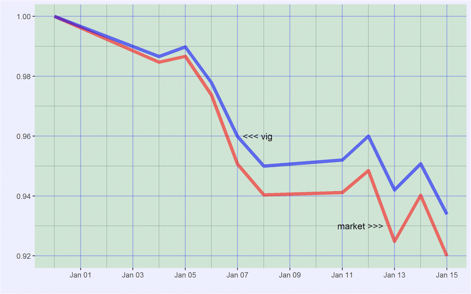
As far as the current (early 2016) market malaise goes, not surprisingly, dividend growth stocks are outperforming the market. Admittedly, they are getting hit but these are high-quality companies and they are not getting hit nearly as much as many other segments of the market, or the market itself:

An important tenet of Investing in Dividend Growth Stocks (Amazon) is that dividend growth stocks are core holdings because they generate good long-term risk-adjusted returns. They do so through a combination of moderate returns and relatively low volatility. Quoting from page 20:


"[A] portfolio [of dividend growth stocks] rises less than the market during bull markets and falls less than the market during bear markets. The latter more than makes up for the former. These stocks march to the beat of a different drummer -- but a very sensible one."



In my opinion, these stocks are excellent long-term investments (subject to not paying too much, as always, of course) for anyone who wants to preserve and build their wealth.


These are not gimmicky companies or slow-growth companies or risky companies. These are companies that last. They grow moderately over long periods, which when combined with relatively low return volatility results in strong gains in long-term wealth.

Probabilities for the S&P 500 weekly return

The previous post highlighted the relative rarity of 2016's week 1 return in the context of history. The following plot shows this in another way. It shows the probability density function (Wikipedia) for the S&P 500 weekly return based on history:

The green area highlights areas where the weekly return is positive; the red area highlights areas where the weekly return is less than -5 percent; and the blue area highlights the in-between areas.

With this probability density function, we deduce probabilities for the S&P 500 in any given week:

• Probability of S&P 500 returning less than -10 percent in a week is 0.1 percent.
• Probability of S&P 500 returning less than -5 percent in a week is 1.4 percent.
• Probability of S&P 500 returning less than -2 percent in a week is 12.5 percent.
• Probability of S&P 500 returning less than -1.5 percent in a week is 17.9 percent.
• Probability of S&P 500 returning less than -1 percent in a week is 25.3 percent.
• Probability of S&P 500 returning less than -0.5 percent in a week is 33.2 percent.
• Probability of S&P 500 returning less than 0 percent in a week is 43.5 percent.
• Probability of S&P 500 returning less than 0.5 percent in a week is 54.9 percent.
• Probability of S&P 500 returning less than 1 percent in a week is 66.5 percent.
• Probability of S&P 500 returning less than 1.5 percent in a week is 77.9 percent.
• Probability of S&P 500 returning less than 2 percent in a week is 85.1 percent.
• Probability of S&P 500 returning less than 5 percent in a week is 98.6 percent.
• Probability of S&P 500 returning less than 10 percent in a week is 99.9 percent.

The second bullet agrees with the observation of the previous post, that the S&P 500 losing more than 5 percent in a week is about 1 in 70, or about 1.4 percent.

According to the  seventh bullet, the S&P 500 suffers a down-week 43.5 percent of the time. Consequently, the S&P 500 encounters an up-week 56.5 percent of the time. This fits the conclusion of an earlier post about daily returns -- that the market closes up on any given day about 53.7 percent of the time (though that post was based on a different set of data). Weekly returns show positive closes with a slightly higher up-probability than daily returns because of compounding. In fact, this logic works sequentially for all types of returns -- thus monthly returns have higher up-probabilities than weekly returns, annual returns have higher up-probabilities than monthly returns, five-year returns have higher up-probabilities than annual returns, and so on.

I zoomed in on the red area, where life is unpleasant:

If you are unfamiliar with probability density functions, here is the same data shown as a histogram. A histogram sorts the data and organizes it into buckets with the height of each bucket, in this plot, a count:

And a zooming-in of the nasty left tail shows the location of the first week of 2016:

Portfolio returns versus risk, a spreadsheet model to calculate portfolio beta

The punch line: Weigh your portfolio's performance, that is your returns, against the risk that you are taking.

---

Beta is not an ideal measure of risk but when looking at how your portfolio fluctuates from day to day it isn't bad. It certainly measures how much your stock moves relative to the market -- and you can use this fact to gauge what the market thinks of your stock.

---

This is especially important if you have an aggressive portfolio and the market is weak. You don't want to panic and sell foolishly. For example, suppose your aggressive portfolio's beta is 1.5. Suppose the market falls seven percent. (It can be a daily fall or a multi-period fall.) Then your portfolio should be expected to fall 1.5 * 7 or 10.5 percent. Now, if during a market fall, your portfolio falls "only" (say) 5 percent, that's not bad. You are outperforming the market relative to the risk that you are taking. If, on the other hand, your portfolio falls (say) 15 percent, that's bad. You are underperforming the market relative to the risk that you are taking.

You might think that a fall of 5 percent is bad. You lost money. And in that sense it is. But you cannot be expected to never lose money and always earn money! What you are hoping for instead is that you are more than compensated for the risk that you are taking. What you are hoping for is that the smaller fall in your portfolio value relative to the market during downturns implies that you've got good individual stories. Holders in your stocks believe in these stories and are not willing to sell during market downturns. Over the longer term, these better-than-expected stories should lead to better-than-average returns.

---

Here's a spreadsheet that shows how to calculate your portfolio's beta using Excel:

The spreadsheet is straightforward. It uses the result from here, http://www.neocadence.com/2013/06/calculating-beta-of-portfolio.html, that is, the beta of a portfolio is the sum of its weighted betas.

Column C lists your positions.
Column D lists how much you have in dollars in each position.
Cell D24 is the total value of your portfolio, the sum of the individual values.
Column E are the percentages, or weights, equal to the values in Column D divided by D24.
Column G lists the betas. You can get these from a site such as Yahoo! Finance.
Column H are the weighted betas, equal to Column E times Column G.
Cell H24 is your portfolio's beta, the sum of the weighted betas.

(The beta for cash is zero. You can include mutual funds and ETFs here as well.)

---

If your portfolio falls less than what is expected, you've got individual stories that are trumping the market's weakness. That's good -- you've got so-called positive alpha. If your portfolio falls more than what is expected, you've got individual stories that are playing out worse than the market's weakness. That's bad -- you've got so-called negative alpha.

Calculating the beta of a portfolio

The punch line: The beta of a portfolio is the sum of its weighted betas.

---

It is not difficult to see why.

Beta, as originally defined by I believe Sharpe sometime around 1962, is the slope of a linear regression line when the market's excess return is plotted on the x-axis and the stock's excess return is plotted on the y-axis.*

---

Accordingly, per the formula for the slope of a linear regression line:

\[ \beta=\frac{Cov\left(r,R\right)}{Var(R)} \]

Here, Cov stands for covariance and Var for variance. The lower-case r is for the stock and the upper-case R is for the market.

---

For a portfolio of two stocks, A and B, because the return of a portfolio is the sum of its weighted returns, the formula becomes:

\[ \beta=\frac{Cov\left(w_{a}r_{a}+w_{b}r_{b},R\right)}{Var(R)} \]

Here the w's represent the weights of each stock in the portfolio. For example, if a portfolio is 70% IBM and 30% JNJ, the weights are 0.7 for IBM and 0.3 for JNJ.

---

Conveniently, because the covariance function is linear in its arguments, in particular its first argument:

\[ \beta=\frac{w_{a}Cov\left(r_{a},R\right)+w_{b}Cov\left(r_{b},R\right)}{Var(R)} \]

Or:

\[ \beta=\frac{w_{a}Cov\left(r_{a},R\right)}{Var(R)}+\frac{w_{b}Cov\left(r_{b},R\right)}{Var(R)} \]


Or:

\[
\beta=w_{a}\beta_{a}+w_{b}\beta_{b}

\]

---

In other words, the beta of a portfolio of two stocks is the sum of its weighted betas. The result extends to three or more stocks and, indeed, to not just stocks but to any assets -- as long as the definition of beta makes sense.

---

To see how this works in real life, suppose you own a portfolio, 70% of which is in IBM, with a beta of 0.7, and 30% of which is in JNJ, with a beta of 0.5. The weighted beta for IBM is 0.7 * 0.7 or 0.49. The weighted beta for JNJ is 0.3 * 0.5 or 0.15. The beta for the portfolio is the sum of the weighted betas, that is, 0.49 + 0.15, or 0.64. Piece of cake, right?

---

* Excess return is return over and above the return of a risk-free asset. In other words, excess return of an asset is the return of the asset minus the return of a risk-free asset. If a stock's return is 5% and a risk-free asset's return is 1%, the stock's excess return is 4%.

When stock prices fall

If a stock with a low standard deviation of returns falls by a small amount then in some ways that is equivalent to a much larger fall in a stock with a higher standard deviation of returns.

Why?

True, ipso facto, you lose less when anything falls less...

But that's not the point here....

What is interesting is that from a probabilistic point of view, a stock with a standard deviation of returns of (say) half that of another stock is falling the "equivalent" amount, again in a probabilistic sense, when it falls half as much as the second stock.

In other words, when you buy a stock, you're not just buying the return, you're also buying the risk.

Calculating your portfolio's delta

Because deltas are nothing but (partial) differentiation operators, and differentiation operators add in the natural way, deltas also add in the natural way. Thus, the delta of a portfolio is the sum of the deltas of the pieces of the portfolio:

\[ \delta_{P}=\sum_{i}w_{i}\delta_{i} \]

Here, $\delta_{p}$ is the delta of the portfolio, $w_{i}$ are the weights of the components of the portfolio, and $\delta_{i}$ are the deltas of the components of the portfolio.

For example, suppose you have a portfolio made up of a stock and call and put options on the stock, as follows:

• 25 percent in the underlying stock.
• 40 percent in call options on the underlying stock, each with a delta of 0.6.
• 35 percent in put options on the underlying stock, each with a delta of -0.3.

Because the delta of a stock is 1, the delta of your portfolio is:

0.25 * 1 + 0.4 * 0.6 + 0.35 * (-0.3)

or

0.385.

In other words, using the implications of the definition of delta, as noted here, your portfolio moves 38.5 percent of the move in the underlying stock.

---

Additional material: To understand the essence of delta hedging, read this.

More on the Mean-Variance Portfolio, 1995 to 1999, stocks vs. bonds

More on the 1995-1999 Mean-Variance portfolio, a picture of which was posted earlier, and is reproduced above.

The Mean-Variance Portfolio, stocks vs. bonds, 1995 to 1999, was a fairly ridiculous 90% stocks plus 10% bonds. Compared to today's returns -- and the typical returns in the stock market -- the expected return from this portfolio is absurd: 25%. Risk is absurdly low as well: 5.53%.

The high concentration in stocks in the Mean-Variance portfolio was because (1) stocks performed so exceptionally well during this period;  (2) they did so with relatively low risk; and (3) bonds and stocks were highly correlated.

Stocks averaged returns of 27% a year with risk of just 5.5%. Bonds actually had lower returns, 7.8% a year, and with somewhat higher risk, 6.4%. In addition, adding bonds to stocks added very little -- there was no significant diversification effect: Bonds and stocks were correlated to the tune of 84%.

Stocks did very well during this period because of the internet mania in tech stocks, upgrades to computer systems in anticipation of Year 2000 problems, and the release of liquidity by the Fed in anticipation of a Year 2000 collapse that did not come. Buy on the dip worked then.

Delta Hedging

Consider a portfolio with exactly one share of a stock, value S. How do you protect it from small moves in S? That is, how do you keep the value of your portfolio stable when S changes by a small amount? The answer: You buy insurance. Translated: You take a position (usually, in an option) which moves in the opposite direction of S. Then when S moves one way, the option will offset it with a move in the other way. With the right number of units of the option, your portfolio will now be stable. But what is the right number of units of the option? There's where delta hedging comes in.

In an earlier post, we saw that delta is defined by:

$$\Delta =\frac{\partial f\left(S,\mathrm{...}\right)}{\partial S}$$

Writing this in the form of infinitesimals, we get:

$$\Delta =\frac{\delta f}{\delta S}$$

Transposing the infinitesimal of S with delta:

$$\delta S=\frac{1}{\Delta }\delta f$$

Or, on moving the right-hand-side term to the left:

$$\delta S-\frac{1}{\Delta }\delta f=0$$

In other words, when S changes by a small amount, a number of units of [-1 divided by delta] of f will ensure that your portfolio does not change in value. It is protected. (That's what the 0 means. The change in portfolio value is zero.)

----

As an example, suppose you have one share of IBM and you want to delta-hedge it. You are thinking about hedging it with IBM call options each with a delta of 0.5. How many call options do you need? Answer: You need (-1/0.5) or -2. Thus, you need to short 2 call options. Easy, right?

----

To summarize: To delta-hedge each share of stock that you hold, you need a position of [-1 divided by delta] units of the option. If the minus sign throws you off, think of the number of units as [1 divided by delta] and set the sign mentally to make the net change equal to 0. Thus, in the IBM example, you need to short the option because you need a negative sign to offset the positive position in the stock.

Delta

Delta is one of the infamous Greeks of Modern Portfolio Theory.

It is the most straightforward of the Greeks, however, being the partial derivative of an option (future, or whatever) with respect to the underlying (here, stock price):

\[ \delta=\frac{\partial f(S,...)}{\partial S} \]

As a (partial) derivative, delta indicates how much the option moves when the underlying moves.

For instance, an option with a delta of +0.3 moves 30 percent of the underlying in the same direction. If the underlying moves up 20 percent, the option moves up 6 percent; if the underlying moves down 20 percent, the option moves down 6 percent.

Conversely, options with negative deltas move opposite to the direction of the underlying: They move down when the underlying moves up and up when the underlying moves down.

Because of this neat little trick, options with negative deltas form the basis of hedging.

Feasible set and mean-variance portfolio, stocks vs. bonds, 1993 to 2010

Normally, you'd expect a much higher contribution from stocks. Not so between 1993 and 2010.

If you could magically look back and forecast, the optimal portfolio was 97 percent in bonds and just 3 percent in stocks. How's that for Stocks for the Long Run, Mr. Jeremy J. Siegel!

The shape of the curve is also quite strange. Normally you'd expect something like a U-shaped curve rotated 90 percent clockwise and funneling wide to the right. I'll have to check all of this at some point, because I find it hard to believe, but I think it's right.

Mean-variance portfolio, 1995-1999, stocks vs bonds